Functions of several variables
Visualization:
the n-dimensional real space
Definition
Let D be a subset of
The graph of a function on
Definition
Let
- The graph of a function of n variables is a subset of (n + 1) dimensional real space
- The graph of a function of 2 variables is a surface in
Level curves
Definition
Let
- the level curve can also be called a contour line
Limits of functions on
- limit laws work the same way.
- The replacement rules are similar (instead of an interval surrounding c, use an open circular disc with center c)
- there is a sandwich info.
- definition and properties of continuity are automatically inferred.
Continuity:
Definition
Let
Practical approach:
- f(c) exists (c lies in the domain of f)
exists (f has a limit as x approaches c) - (check that the limit equals the function value)
Path limits
- Difference to functions of one variable: there are no one sided limits.
Definition
A path limit is the limit of f(x) where x approaches c along a continuous path ending in c.
info
The following statements are equivalent:
- (i) The limit
exists - (ii) All path limits of f(x) along continuous paths ending in c exist, and have the same value.
WARNING
In order to conclude i from ii you must show that path limits exist. and are the same along every possible path.
Showing that a limit does not exist:
info
- If a path limit along a continuous path ending at c does not exist, then
does not exist. - If two paths limits along continuous paths ending at c do exist, but they are not the same then
does not exist.
Polar coordinates:
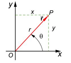
- Every point (x, y) is described by two polar coordinates r and
- The number r is called the radius, and is defined as the distance to (0, 0)
- the number
is called the polar angle, and is defined as the angle between the vector r and the positive x-axis.
Coordinate transformation:
- From polar coordinates to Cartesian coordinates:
- From Cartesian coordinates to polar coordinates:
Limits and polar coordinates:
info
Let f be a function of two variables.
If, after transformation to polar coordinates, f(x, y) can be written in the form:
with:
bounded function.
then:
- If the two requirements are not satisfied the limit most likely does not exist.
Partial Derivatives
Definition
- The partial derivative of f with respect to x at (x0, y0) is:
- The partial derivative of f with respect to y at (x0, y0) is:
How to calculate partial derivatives:
- The partial derivative with respect to x is the derivative of the function f(x, y) where y behaves like a constant.
- The partial derivative with respect to y is the derivative of the function f(x, y) where x behaves like a constant.
Higher Order Partial derivatives of f:
Mixed higher order partial derivatives:
Mixed Derivative info
If f(x,y) and it's partial derivatives exist and are continuous on an open environment of (a, b) then
Linearization
The tangent plane
The tangent plane V at
is spanned by the vectors and A normal vector is
A normal equation for V is
or
Definition
The tangent plane is the graph of the linear function
- this function is the linearization of f at (x0, y0)
- The function L is an approximation of f in the neighborhood of (x0, y0)